Juan Carlos Espinosa Ceniceros: Teoría de la Información

Mostrando entradas con la etiqueta Teoría de la Información. Mostrar todas las entradas

domingo, 26 de mayo de 2013

[IT] Card game extra points 2

Dynamic: "Dynamic dictionaries are constructed from the input and are embedded into the coded message."
Exhaustive: "Write a program and perform some exhaustive tests."
Parity: "The parity bits that permit detecting and correcting a single-bit error."
Similarity: "Sequence similarity usually implies functional similarity."
Conditional: "Choose that code word that has the highest conditional probability given the received sequence, in terms of the transition probabilities.."
Lookahead: "Based on a sliding-window technique using a lookahead.."
Prefix: "A prefix is an affix which is placed before the root of a word."
Analysis: "A real function will now be represented by a combination of other real functions, for those that dislike complex analysis."
Encoding: "The program consists in the commented source code for both encoding and decoding ASCII text."
Incomplete: "If there are collisions of two or more symbols yielding the same value, this is called an incomplete MLD."
Metric: "A metric or distance function is a function that defines a distance between elements of a set."
Occurrence: "."Tornado occurrence by hour of day for the United States
Global: "Published in some global manner so that all who encode or decode have access to them. "
Tree:"Computation tree is a representation for the computation steps of a non-deterministic Turing machine on a specified input."
Wavelet: This can be done as a Fourier, cosine, or sine transform, or with wavelets as we discussed in computer vision.
Precomputed:"There are some precomputed mathematical tables of common logarithms."
Average: "The average error probability E = 1 - R."
Sequence:"Choose that code word that has the highest conditional probability given the received sequence, in terms of the transition probabilities."
Distance:"R-S codes maximize the minimum distance between code words among all linear codes that use the same input/output block sizes"
Access:"Published in some global manner so that all who encode or decode have access to them."
Adaptive: "Invent, implement, and evaluate your own adaptive coding method."
Message: "Error-correcting codes are designed to recover from one or more transmission error and allow determining what code word the message corresponds to even in the presence of errors."
Frequency: "No frequency calculations are possible in the beginning."
Periodic: "We can represent periodic signals as summations of complex exponential functions; this is the Fourier transform."
Correction: "Error correction methods"
Reliability: "Reliability is the ability of a person or system to perform and maintain its functions in routine circumstances"
Fourier: "We can represent periodic signals as summations of complex exponential functions; this is the Fourier transform."
Concatenate: "The concatenate function allows you to join 2 or more strings together."
Transmit: "The channel is used to transmit the messages..."
Quantize: "To compress, we may ignore or quantize some of the frequencies present according to some criteria."

jueves, 9 de mayo de 2013

[IT] Homework 5: Error detection (Hamming Block Code)

For this week we had to implement an error detection technique using a block code method. We had to simulate the transmission of data through a noisy channel and use our error detection technique to fix the errors during the transmission.
I use the Hamming Code as my block code method.

NOTE: If you want to understand how works the Hamming Block Code, check the references at the footer.

Experiment

For my experiment, I prepared a Python script that generate several random words of length 4 (4 bits) and then, send them through a noisy channel, the parameters of the experiment are:

wordLength: Word length (4 bits)
frecZeros: Frequency of zeros in the word
probError: Probability that a word is transmitted wrong by the channel
errorBits: Maximum number of errors in the transmitted word
rep: Amount of experiment repetitions

For the experiment, the wordLength and the errorBits are fixed at 4 and 1, respectively, the parameters freqZeros and probError only affects the final behavior of the channel.

As we can see, with 1 as the number of error bits in the word, the Hamming Block code can fix all the errors without problems.

If we increase the amount of erros in each word, for instance, 2 errors per word, we begin to experience some failures in the method

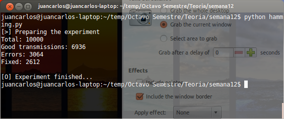
There are not much difference if we increase the amount of errors to 3

The Hamming Code methos works fine while the amount of errors in a word still's one, but, when the amount of errors increases two a number bigger than one, the Hamming Code will start to experiment some failures.

Also,we can see that the amount of good transmissions and errors follows a linear relation.

The implemented Hamming Code uses a 7x4 "H" matrix, with which is able to correct a single bit error.

When you multiply the original 4-bits word and the encode "G" matrix, the result is a 7-bit codeword "xG":

When you decode the codeword using the "H" matrix, the multiplication result is a 3-bit word. That word is a binary representation of a single digit. The digit represents the bit that is wrong in the transmitted codeword through the noisy channel.

We only need to translate the binary representation to an integer, which we will be able to correct the bit error.

Code

References:

Michael Dipperstein, Hamming (7,4) Code Discussion and Implementation, extraído de: http://michael.dipperstein.com/hamming/
Encoding and Decoding with the Hamming Code, extraído de: http://www.uwyo.edu/moorhouse/courses/4600/encoding.pdf

jueves, 25 de abril de 2013

[IT] Extra points: Dictionary based encoding

Un método de codificación que encontré para está actividad se llama Byte-Pair encoding.

Es uno de los métodos por diccionario más simples que existen.

El procedimiento es muy simple, cuando se encuentran un par de bytes consecutivos y ducho par se repite varias veces en el texto, entonces dicho par de bytes es reemplazado por un byte que no se éste utilizando.
El algoritmo se detiene cuando ya no hay más pares de bytes consecutivos.
Es necesario almacenar el diccionario para poder recuperar la información

Ejemplo

Codificación

Iniciamos con una cadena de caractéres, con un largo aleatorio, por ejemplo

dcbdbdababdbacbbdabaaaacacacaa

Nuestro alfabeto sería:

alpha = [a,b,c,d]

Por lo que tenemos los bytes desde "e" hasta "z" si quitamos los caractéres de control y signos de puntuación.

Comienzamos a recorrer la lista para buscar por pares de caractéres:

Iteración 1: Encontramos el par que más se repite bd, asignamos un byte no utilizado:

bd : e

Identificamos:

d c b d b d a b a b d b a c b b d a b a a a a c a c a c a a
     e   e                     e

Sustituimos:

d c e e a b a b d b a c b e a b a a a a c a c a c a a

Iteración 2: Encontramos el par que más se repite ab, asignamos un byte no utilizado:

ab : f

Identificamos:

d c e e a b a b d b a c b e a b a a a a c a c a c a a
         f   f               f

Sustituímos:

d c e e f f d b a c b e f a a a a c a c a c a a

Iteración 3: Encontramos el par que más se repite ca, asignamos un byte no utilizado:

ca : g

Identificamos:

d c e e f f d b a c b e f a a a a c a c a c a a
                                   g   g   g
Sustituímos:

d c e e f f d b a c b e f a a a a g g g a

Iteración 4: Encontramos el par que más se repite aa, asignamos un byte no utilizado:

aa : h

Identificamos:

d c e e f f d b a c b e f a a a a g g g a
                           h   h

Sustituímos:

d c e e f f d b a c b e f h h g g g a

Iteración 5: Encontramos el par que más se repite, aqui encontramos varios pares que se repiten solo una vez (ee, ff, hh, gg), asignamos un byte no utilizado a cada una:

ee : i
ff : j
hh : k
gg : l

Identificamos:

d c e e f f d b a c b e f h h g g g a
     i   j                 k   l

Sustituímos:

d c i j d b a c b e f k l g a

Como ya no hay bytes juntos que se repitan, entonces podemos terminar la ejecución, los resultados serían:

dcbdbdababdbacbbdabaaaacacacaa = 30 carácteres
dcijdbacbefklga = 15 caractéres.

Y el diccionario quedaria

bd : e
ab : f
ca : g
aa : h
ee : i
ff : j
hh : k
gg : l

Decodificación

Para la decodificación, primeo debemos girar el diccionario y ordenarlo de forma inversa para buscar por las coincidencias hasta que no encontremos ninguna más:

Cadena original: dcijdbacbefklga

Identificamos: l
Sustituimos por: gg

d c i j d b a c b e f k l g a

Queda:

d c i j d b a c b e f k g g g a

Identificamos: k
Sustituimos por: hh

d c i j d b a c b e f k l g a

Queda:

d c i j d b a c b e f h h g g g a

Identificamos: j
Sustituimos por: ff

d c i j d b a c b e f h h g g g a
Queda:

d c i f f d b a c b e f h h g g g a

Identificamos: i
Sustituimos por: ee

d c i f f d b a c b e f h h g g g a

Queda:

d c e e f f d b a c b e f h h g g g a

Identificamos: h
Sustituimos por: aa

d c i f f d b a c b e f h h g g g a

Queda:

d c e e f f d b a c b e f a a a a g g g a

Identificamos: g
Sustituimos por: ca

d c e e f f d b a c b e f a a a a g g g 

Queda:

d c e e f f d b a c b e f a a a a c a c a c a a
Identificamos: f
Sustituimos por: ab

d c e e f f d b a c b e f a a a a c a c a c a a

Queda:

d c e e a b a b d b a c b e a b a a a a c a c a c a a


Identificamos: e
Sustituimos por: bd

d c e e a b a b d b a c b e a b a a a a c a c a c a a

Queda:

d c b d b d a b a b d b a c b b d a b a a a a c a c a c a a

Y asi se hace el deflate de los datos.

Referencias:

[PDF] Byte pair encoding: a text compression scheme that accelerates pattern matching.

Yusuke Shibatay,

Masayuki Takeday,

Takuya Kiday, Shuichi Fukamachiz,

Ayumi Shinoharay, Takeshi Shinoharaz,

Setsuo Arikaway

Dept. of Informatics, Kyushu University 33, Fukuoka 812-8581, Japan

f yusuke, kida, takeda, ayumi, arikawag @i.kyushu-u.ac.jp

Dept. of Arti cial Intelligence, Kyushu Institute of Technology, Iizuka 320-8520, Japan

f fukamati, shinog @ai.kyutech.ac.jp

[IT] Homework 4: Adaptative methods

For the homework of this week, we had to design an algorithm to turn our implementation of Huffman's Coding into an adaptative implementation of Huffman's coding.

...

Hipotesis

Since the Huffman's coding needs to build a binary tree, there is a possibility to improve the three construction.

So, my approaching is to improve the tree construction everytime when a new node is added to it.

A common Huffman's coding tree looks like tihis:

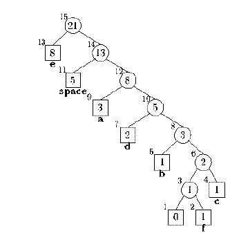
When the structure of the tree is too deep, we will get very large huffman codes for the less frequent letters.

Maybe, rebalancing the tree in each run, shorters codes could be generated and a little more space could be saved.

So, my approaching is center the huffman's coding in the frequencies of the character to reconstruct and rebalance the tree in each run and get a structure like this:

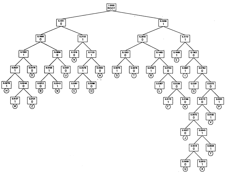
Where we can get more and shorter codes.

It's expected that this implementation will be more resource and time expensive, but also it's expected that the final results will be better.

...

There is no code :(

I don't have enough time to complete the homework this time, I hope don't fail with the other ones.

domingo, 7 de abril de 2013

[IT] Card game extra points

Label: "Label all edges heading to the right with a zero and those heading to the left with ones."
Column: "Initialize the first column of M all zero if the first character of the text is not equal to the first character of the pattern."
Binary: "For binary text and a binary pattern"
Rule: "Special rules to save more time by shifting more positions: Bad character rule, Good suffix rule"
Efficient: "Knutt-Morris-Pratt, usually less efficient, but much easier to explain and prove."
Pattern: "
When a substring of the pattern aligns and then there is a mismatch
at position i, move the pattern i - sp’ i positions to the right.
Fuzzy: "
Example: binary input, fuzzy or stuttering output
Lossless: "
If all bits of L can be recovered from S, the compression is lossless.
Dictionary: "
The dictionary is included in the beginning of the compressed
file, unless it is implicitly constructed in a standard way
Code word: "
Each word is replaced by a (shorter) code word.
The code words usually cannot share prefixes
Obtain: "
Concatenate the edge labels for the path from the root to a leaf to
obtain the code word for the symbol at that leaf.
Preprocessing: "
The use of shortcut rules generally requires preprocessing.
Average: "
Average information content:
Logarithm: "
The base of the logarithm is not that crucial; interpret it as units,
base two being the bit (binary digit)
Root: "For any leaf i, the labels on the path from the root to that leaf concatenate to exactly the suffix S[i..m]."
Symbol: "
An implicit suffix tree for S is obtained from a suffix tree by
removing the terminal symbol $ from all edge labels, removing
any unlabelled edge, and removing subsequently all nodes that
do not complete at least two children.
Equal: "
If the two are equal for a given r and P is of length n, then there is
a match to P starting at r in T."
Worst case: "
How does this differ from the worst case complexity?
Rate: "
The rate of information flow; the maximum value of...
Compute: "To compute M( j ), we perform a binary AND on Bit-Shift( j -1) and U ( T ( j ) )."
Correct: "
The probability of correct transmission is denoted as p
Optimal: "
Optimal input frequencies
Buffer: "
Online compression = the string arrives bit by bit,
possibly with a limited-capacity buffer
Apply: "
We must apply mod p during the computations of the H values
for this to save us anything at all.
Complexity: "
Install and experimentally determine the “typical-case”
complexity.

jueves, 4 de abril de 2013

[IT] Homework 3: Text compression

For this homwork, we had to implement the tree-based Huffman's encoding for unicode strings.

Also, we had to design, document, and analyze an experiment to determine the worst-case and typical-case complexity and compression ratio.

Huffman's coding

The Huffman encoding algorithm is an optimal compression algorithm. In this algorithm only the frequency of each individual letters are used to compress the data.

The main idea is that if the text have some letters that are more frequent than others, then that letters can be represented by fewer bits to encode those letters than to encode the less frequent letters.

For instance, if you have the string:

"I ate an apple"

We can get the frequencies of each letter and build a hash table:

Letter	Frequency	Encoding representation
a	3	00
e	2	110
i	1	1010
n	1	1000
p	2	111
t	1	1001
l	1	1011
space	3	01

Originally, each characters is represented by a byte, so, if our string have 14 characters then the size is 14 bytes or 112 bits.

Using the new encoding representation, the string is represented in that form:

010100100011110001001111001001011011110110

|0101|00   |100|011|110|00   |100|1111|00   |100|101|101|1110|110|
i    space a   t   e   space a   n    space a   p   p   l    e

Requiring only 46 bits, so, we can calculate a compress ratio of 38% or 1 to 2.6 , with a space saving of 62%.

In fact, each binary ecoding representation is a path in a binary tree, each bit represents the direction where we must to search to find a letter (left or right, 0 or 1) and the length of the binary representation means which deeper we must to search to find the letter.

If you want to know more of the background of Huffman's encoding algorithm, I recommend the following links:

http://www.cprogramming.com/tutorial/computersciencetheory/huffman.html

http://www.youtube.com/watch?v=ZdooBTdW5bM

Experiment

Basically what I did was to program two Python's scripts.

The first one performs the Huffman's encoding algorithm. That scripts follows these steps for compression:

Receive the path to the text file.
Reads the file and calculate the frequencies of each character.
Build the binary tree.
Get the binary representation of each character walking through the paths of the tree.
Compress the text using the new binary representation of each characters.
Calculates:

the time of the compression process
the text size before and after compression
the memory used during the compressio (tree size)
the compress ratio and the space savings

And these steps for decompression:

Receive the path to the compressed file and the dictionary file.
Loads the dictionary on memory.
Reads the compressed file char by char searching on the dictionary for the binary-like string representation.
Changes the binary-like string representation for the corresponding letter.
Calculates:

the time of the decompression process
the text size before and after decompression
the memory used during the decompression (doctionary size)
the compress ratio and the space savings

The second script builds the experiment environment, passing the text files to the first script and receiving all the calculated data from the first script.

Each text is compressed/decompressed 30 times and an AWK script calculates the average time, memory and compress ratio for each case.

The results are saved on plain text file separated by spaces, in order to be plotted later using Gnuplot.

For the experiment I ran two cases

The typical one where I used twenty (20) chapters of "Don Quixote de la Mancha" in 3 different sizes
The worst one where I generated twenty (20) texts with an uniform frecuency of characters, using random functions, in 3 different sizes.
The sizes of the files was:

Small = 10000 characters
Medium = 50000 characters
Big = 100000 characters

Results

A) Compression case

Time

Typical / Time

Worst / Time

As we can see in the pictures, the typical case is faster than the worst time, but only by few miliseconds.

Also, in this case, we can see that the size of the texts doesn't affect the performance of the algorithm because the time grows linearly with respect the size of the text.

Also, there are some fluctuations over the compression of each text in each size case, maybe this happens because the computer has more processes in memory, you can see in the graphs that the fulctuations has some pattern due the computer usage while the algorithm was running.

Memory

Typical / Memory

Worst / Memory

The memory aparently doesn't change too much in every case, only a a few bytes in every size change.

In the typical case, the size of the tree it's being plotted, in the worst case the size of the dictionary used to decompress the text it's being plotted.

While the size of the dictionary it's the same in each text size for the worst cases, the size of the tree grows in the typical case, but doesnt have a signifficant growth.

Compression Ratio

Typical / Ratio

Worst / Ratio

In this graphs, the data could be a little tricky, as greater than the compression ratio is, the space savings is lower. The compression ratio is measured in a scale from 0 to 1.
In the typical case, the compression ratio is almost the same in all the cases, arround 0.5 or 0.6, so, the --correct interpretation of the compression ratio is write a scale such as 1:2 aproximately. That means arround a 40% - 50% of space savings.

B) Decompression case

For the decompression case, I only plot the time of the process and the used memory.

Time

Typical / Time

Worst / Time

In this case, the time aparently behaves similar to the compression case, but now, the decompression time of the bigger texts is greater than in the compression case.

But in this cases, the time appears to grow also linearly when the text size grow.

Memory

Typical / Memory

Worst / Memory

Also, the memory appears to be consistent in each case, and doesn't fluctuates very much in each repetition. The more significant change is in te typical case, in the jump from 10000 characters to 50000 characters. Apparently, the text size could have a more remarkable effect in the decompression process than the compression process.

Conclusion

In conclusion, we can say that:

In the time, as great is the compression/decompression text, the time is also greater, but the time grows linearly.
The memory appears to not grow to much, the most significant growth is when we jump from small texts to medium texts.
The compression ratio doesn't change to much in each text, but, we espect that when the size text grows, the compression ratio is lower and the space savings are greater.
The performance of the algorithm is only affected in time, when the text size grows.

Code

Algorithm

Experiment builder

Awk postprocessor

References:

jueves, 21 de febrero de 2013

[IT] Homework 2: Coupling text methods: Boyer-Moore & Knuth-Morris-Pratt

Implementation of Knuth-Morris-Pratt and Boyer-Moore algorithms in Python, written by me:

Execution

This is the code to automate all the execution:

Experiment

My initial conditions was:

Word length: from 100 to 1000
Pattern length: from 2 to 11
Repetitions: 30

I made all the posible conditions between these values, iterating the pattern length through each word length, and also running each combination 30 times.

Results

Knuth-Morris-Pratt
Time	Comparisons

Boyer-Moore
Time	Comparisons

I wrote these codes after understanding the following examples:

http://www.inf.fh-flensburg.de/lang/algorithmen/pattern/kmpen.htm
http://www-igm.univ-mlv.fr/~lecroq/string/node8.html
http://www-igm.univ-mlv.fr/~lecroq/string/node14.html

martes, 12 de febrero de 2013

[IT] Traducción

Contribuí en la traducción del documento:

A Mathematical Theory of Communication

del autor C. E. Shannon.

Se me asignaron las páginas 36 a 40.

El archivo con la traducción es juan.tex, ubicado en el repositorio

TraduccionShannonPaper

domingo, 10 de febrero de 2013

[IT] Homework 1. Noisy channel simulation

The activity of this blog entry was to program some scripts to simulate the transmision of some random information through a Binary Symmetric Channel. Also we have to analyze the final results of the simulation

Basically what I did was to program a script in Python to generate the necesary parameters to run the simulation, the parameters are:

Word length (binary word)
Maximum length of the words
The length of the word traduced in power of two
Quantity of words of the same size
The numbers of repetitions of transmit a word throught the binary symmetric channel
Frecuency of appearance of zeros in each word
The probability that a zero continues being a zero after the transmission
The probability that a one continues being a one after the transmission.

My initial conditions was:

Parameter	Value
Word length	1
Max. word len.	1024
Power of two	from 0 to 10
Zero frecuency	[from 0.1 to 0.8]
Probability of zeros	[0.45, 0.55, 0.70, 0.80, 0.95]
Probability of ones	[0.3, 0.60, 0.80, 0.95, 0.90]
Repetitions	30
Quantity of words	30

After that, I was generated all the possible combinations of parameters. I build that in a Python script.

The simulation follows these steps:

The Python simulation script receives the parameters length of word, frecuency of appearance of zeros in each word, the probability of zeros, the probability of ones, the number of repetitions of transmission of each word.
The script builds a word of length "l" containing only zeros and ones (bits).
The script takes that word and simulates the transmission of the word throught a binary symmetric channel, here is where the probabilities of zeros and ones works, sometimes changing some bits. This action is repeated "r" times.
In each transmission the script compares the receives word with the transmitted word, counting only the ocurrences where both words are the same.
The scripts calculates an average with the number of repetitions and the number of a successfull transmissions.
The script returns the calculated average.

After that, another Python script takes the calculated average and writes the value on a temporal file, this process is repeated depending on the amount of words of each length that will be generated, in this case, 30 words. This means that 30 words will be transmitted 30 times each through the channel.

The scripts changes the value of the frecuency of zeros after 30 words with 30 repetitions each, in each change, a script written in awk calculates the average and the standard deviation of each run and saves the result on a special file with special format to plot the results with gnuplot.

Code

Python script that automate all the simulation process:

Python script that simulates the binary symmetric channel:

Awk script that calculates the average and standard deviation in each run:

Results

The purpose of the experiment is to determine the reliability of the channel at different probabilities of zeros and ones, to visualize the results I plot them in a chart using gnuplot. This is the result:

Where the x axis represents the size of the word in powers of two, the y axis represents the different frecuencies of zero, the z axis represents the percentage of a successful transmision through the channel and the color's gradients represents the standard deviation.

As we can see, the reliability of the channel decreases exponentially when the word length increases, with a word length of 5 (32 bits) the reliability of the channel is already below than 20 percent.

Analysis

With a rapid analysis we can recognize the shape of the graph, it's like an exponential function with a negative input and . To provee that I plot each graph in pairs and also I plot the graph of an exponential function, to be more precise, the function:

exp((-x*A)+B)

Where the input x is negative, the input A controls the width of the curve, and the B input displaces the curve on the x axis.

The are the results:

So, we can accurate the behavior of the channel using the function exp((-x*0.6)+4.5), we can't reproduce exactly the behavior of the channel but the exponential function is a good aproximation.

Using the standard deviation, this is the comparison between the analytical function's plot and experimental result's plot:

References